2.8 Efficiency
Decisions of how to represent and process data are often influenced by the efficiency of alternatives. Efficiency refers to the computational resources used by a representation or process, such as how much time and memory are required to compute the result of a function or represent an object. These amounts can vary widely depending on the details of an implementation.
2.8.1 Measuring Efficiency
Measuring exactly how long a program requires to run or how much memory it consumes is challenging, because the results depend upon many details of how a computer is configured. A more reliable way to characterize the efficiency of a program is to measure how many times some event occurs, such as a function call.
Let's return to our first tree-recursive function, the fib function for computing numbers in the Fibonacci sequence.
>>> def fib(n):
        if n == 0:
            return 0
        if n == 1:
            return 1
        return fib(n-2) + fib(n-1)
>>> fib(5)
5
Consider the pattern of computation that results from evaluating fib(6), depicted below. To compute fib(5), we compute fib(3) and fib(4). To compute fib(3), we compute fib(1) and fib(2). In general, the evolved process looks like a tree. Each blue dot indicates a completed computation of a Fibonacci number in the traversal of this tree.
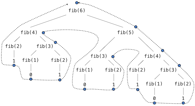
This function is instructive as a prototypical tree recursion, but it is a terribly inefficient way to compute Fibonacci numbers because it does so much redundant computation. The entire computation of fib(3) is duplicated.
We can measure this inefficiency. The higher-order count function returns an equivalent function to its argument that also maintains a call_count attribute. In this way, we can inspect just how many times fib is called.
>>> def count(f):
        def counted(*args):
            counted.call_count += 1
            return f(*args)
        counted.call_count = 0
        return counted
By counting the number of calls to fib, we see that the calls required grows faster than the Fibonacci numbers themselves. This rapid expansion of calls is characteristic of tree-recursive functions.
>>> fib = count(fib)
>>> fib(19)
4181
>>> fib.call_count
13529
Space. To understand the space requirements of a function, we must specify generally how memory is used, preserved, and reclaimed in our environment model of computation. In evaluating an expression, the interpreter preserves all active environments and all values and frames referenced by those environments. An environment is active if it provides the evaluation context for some expression being evaluated. An environment becomes inactive whenever the function call for which its first frame was created finally returns.
For example, when evaluating fib, the interpreter proceeds to compute each value in the order shown previously, traversing the structure of the tree. To do so, it only needs to keep track of those nodes that are above the current node in the tree at any point in the computation. The memory used to evaluate the rest of the branches can be reclaimed because it cannot affect future computation. In general, the space required for tree-recursive functions will be proportional to the maximum depth of the tree.
The diagram below depicts the environment created by evaluating fib(3). In the process of evaluating the return expression for the initial application of fib, the expression fib(n-2) is evaluated, yielding a value of 0. Once this value is computed, the corresponding environment frame (grayed out) is no longer needed: it is not part of an active environment. Thus, a well-designed interpreter can reclaim the memory that was used to store this frame. On the other hand, if the interpreter is currently evaluating fib(n-1), then the environment created by this application of fib (in which n is 2) is active. In turn, the environment originally created to apply fib to 3 is active because its return value has not yet been computed.
The higher-order count_frames function tracks open_count, the number of calls to the function f that have not yet returned. The max_count attribute is the maximum value ever attained by open_count, and it corresponds to the maximum number of frames that are ever simultaneously active during the course of computation.
>>> def count_frames(f):
        def counted(*args):
            counted.open_count += 1
            counted.max_count = max(counted.max_count, counted.open_count)
            result = f(*args)
            counted.open_count -= 1
            return result
        counted.open_count = 0
        counted.max_count = 0
        return counted
>>> fib = count_frames(fib)
>>> fib(19)
4181
>>> fib.open_count
0
>>> fib.max_count
19
>>> fib(24)
46368
>>> fib.max_count
24
To summarize, the space requirement of the fib function, measured in active frames, is one less than the input, which tends to be small. The time requirement measured in total recursive calls is larger than the output, which tends to be huge.
2.8.2 Memoization
Tree-recursive computational processes can often be made more efficient through memoization, a powerful technique for increasing the efficiency of recursive functions that repeat computation. A memoized function will store the return value for any arguments it has previously received. A second call to fib(25) would not re-compute the return value recursively, but instead return the existing one that has already been constructed.
Memoization can be expressed naturally as a higher-order function, which can also be used as a decorator. The definition below creates a cache of previously computed results, indexed by the arguments from which they were computed. The use of a dictionary requires that the argument to the memoized function be immutable.
>>> def memo(f):
        cache = {}
        def memoized(n):
            if n not in cache:
                cache[n] = f(n)
            return cache[n]
        return memoized
If we apply memo to the recursive computation of Fibonacci numbers, a new pattern of computation evolves, depicted below.
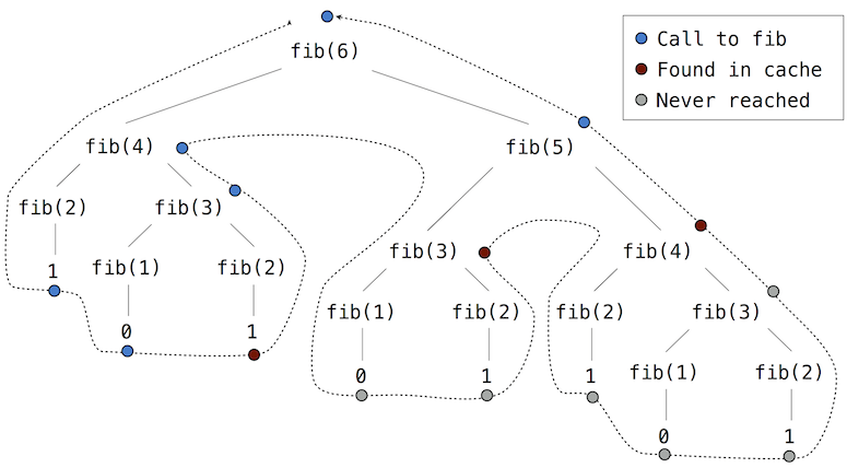
In this computation of fib(5), the results for fib(2) and fib(3) are reused when computing fib(4) on the right branch of the tree. As a result, much of the tree-recursive computation is not required at all.
Using count, we can see that the fib function is actually only called once for each unique input to fib.
>>> counted_fib = count(fib)
>>> fib  = memo(counted_fib)
>>> fib(19)
4181
>>> counted_fib.call_count
20
>>> fib(34)
5702887
>>> counted_fib.call_count
35
2.8.3 Orders of Growth
Processes can differ massively in the rates at which they consume the computational resources of space and time, as the previous examples illustrate. However, exactly determining just how much space or time will be used when calling a function is a very difficult task that depends upon many factors. A useful way to analyze a process is to categorize it along with a group of processes that all have similar requirements. A useful categorization is the order of growth of a process, which expresses in simple terms how the resource requirements of a process grow as a function of the input.
As an introduction to orders of growth, we will analyze the function count_factors below, which counts the number of integers that evenly divide an input n. The function attempts to divide n by every integer less than or equal to its square root. The implementation takes advantage of the fact that if $k$ divides $n$ and $k < \sqrt{n}$ , then there is another factor $j = n / k$ such that $j > \sqrt{n}$.
How much time is required to evaluate count_factors? The exact answer will vary on different machines, but we can make some useful general observations about the amount of computation involved. The total number of times this process executes the body of the while statement is the greatest integer less than $\sqrt{n}$. The statements before and after this while statement are executed exactly once. So, the total number of statements executed is $w \cdot \sqrt{n} + v$, where $w$ is the number of statements in the while body and $v$ is the number of statements outside of the while statement. Although it isn't exact, this formula generally characterizes how much time will be required to evaluate count_factors as a function of the input n.
A more exact description is difficult to obtain. The constants $w$ and $v$ are not constant at all, because the assignment statements to factors are sometimes executed but sometimes not. An order of growth analysis allows us to gloss over such details and instead focus on the general shape of growth. In particular, the order of growth for count_factors expresses in precise terms that the amount of time required to compute count_factors(n) scales at the rate $\sqrt{n}$, within a margin of some constant factors.
Theta Notation. Let $n$ be a parameter that measures the size of the input to some process, and let $R(n)$ be the amount of some resource that the process requires for an input of size $n$. In our previous examples we took $n$ to be the number for which a given function is to be computed, but there are other possibilities. For instance, if our goal is to compute an approximation to the square root of a number, we might take $n$ to be the number of digits of accuracy required.
$R(n)$ might measure the amount of memory used, the number of elementary machine steps performed, and so on. In computers that do only a fixed number of steps at a time, the time required to evaluate an expression will be proportional to the number of elementary steps performed in the process of evaluation.
We say that $R(n)$ has order of growth $\Theta(f(n))$, written $R(n) = \Theta(f(n))$ (pronounced "theta of $f(n)$"), if there are positive constants $k_1$ and $k_2$ independent of $n$ such that
\begin{equation*} k_1 \cdot f(n) \leq R(n) \leq k_2 \cdot f(n) \end{equation*}for any value of $n$ larger than some minimum $m$. In other words, for large $n$, the value $R(n)$ is always sandwiched between two values that both scale with $f(n)$:
- A lower bound $k_1 \cdot f(n)$ and
- An upper bound $k_2 \cdot f(n)$
We can apply this definition to show that the number of steps required to evaluate count_factors(n) grows as $\Theta(\sqrt{n})$ by inspecting the function body.
First, we choose $k_1=1$ and $m=0$, so that the lower bound states that count_factors(n) requires at least $1 \cdot \sqrt{n}$ steps for any $n>0$. There are at least 4 lines executed outside of the while statement, each of which takes at least 1 step to execute. There are at least two lines executed within the while body, along with the while header itself. All of these require at least one step. The while body is evaluated at least $\sqrt{n}-1$ times. Composing these lower bounds, we see that the process requires at least $4 + 3 \cdot (\sqrt{n}-1)$ steps, which is always larger than $k_1 \cdot \sqrt{n}$.
Second, we can verify the upper bound. We assume that any single line in the body of count_factors requires at most p steps. This assumption isn't true for every line of Python, but does hold in this case. Then, evaluating count_factors(n) can require at most $p \cdot (5 + 4 \sqrt{n})$, because there are 5 lines outside of the while statement and 4 within (including the header). This upper bound holds even if every if header evaluates to true. Finally, if we choose $k_2=5p$, then the steps required is always smaller than $k_2 \cdot \sqrt{n}$. Our argument is complete.
2.8.4 Example: Exponentiation
Consider the problem of computing the exponential of a given number. We would like a function that takes as arguments a base b and a positive integer exponent n and computes $b^n$. One way to do this is via the recursive definition
\begin{align*} b^n &= b \cdot b^{n-1} \\ b^0 &= 1 \end{align*}which translates readily into the recursive function
>>> def exp(b, n):
        if n == 0:
            return 1
        return b * exp(b, n-1)
This is a linear recursive process that requires $\Theta(n)$ steps and $\Theta(n)$ space. Just as with factorial, we can readily formulate an equivalent linear iteration that requires a similar number of steps but constant space.
>>> def exp_iter(b, n):
        result = 1
        for _ in range(n):
            result = result * b
        return result
We can compute exponentials in fewer steps by using successive squaring. For instance, rather than computing $b^8$ as
\begin{equation*} b \cdot (b \cdot (b \cdot (b \cdot (b \cdot (b \cdot (b \cdot b)))))) \end{equation*}we can compute it using three multiplications:
\begin{align*} b^2 &= b \cdot b \\ b^4 &= b^2 \cdot b^2 \\ b^8 &= b^4 \cdot b^4 \end{align*}This method works fine for exponents that are powers of 2. We can also take advantage of successive squaring in computing exponentials in general if we use the recursive rule
\begin{equation*} b^n = \begin{cases} (b^{\frac{1}{2} n})^2 & \text{if $n$ is even} \\ b \cdot b^{n-1} & \text{if $n$ is odd} \end{cases} \end{equation*}We can express this method as a recursive function as well:
>>> def square(x):
        return x*x
>>> def fast_exp(b, n):
        if n == 0:
            return 1
        if n % 2 == 0:
            return square(fast_exp(b, n//2))
        else:
            return b * fast_exp(b, n-1)
>>> fast_exp(2, 100)
1267650600228229401496703205376
The process evolved by fast_exp grows logarithmically with n in both space and number of steps. To see this, observe that computing $b^{2n}$ using fast_exp requires only one more multiplication than computing $b^n$. The size of the exponent we can compute therefore doubles (approximately) with every new multiplication we are allowed. Thus, the number of multiplications required for an exponent of n grows about as fast as the logarithm of n base 2. The process has $\Theta(\log n)$ growth. The difference between $\Theta(\log n)$ growth and $\Theta(n)$ growth becomes striking as $n$ becomes large. For example, fast_exp for n of 1000 requires only 14 multiplications instead of 1000.
2.8.5 Growth Categories
Orders of growth are designed to simplify the analysis and comparison of computational processes. Many different processes can all have equivalent orders of growth, which indicates that they scale in similar ways. It is an essential skill of a computer scientist to know and recognize common orders of growth and identify processes of the same order.
Constants. Constant terms do not affect the order of growth of a process. So, for instance, $\Theta(n)$ and $\Theta(500 \cdot n)$ are the same order of growth. This property follows from the definition of theta notation, which allows us to choose arbitrary constants $k_1$ and $k_2$ (such as $\frac{1}{500}$) for the upper and lower bounds. For simplicity, constants are always omitted from orders of growth.
Logarithms. The base of a logarithm does not affect the order of growth of a process. For instance, $\log_2 n$ and $\log_{10} n$ are the same order of growth. Changing the base of a logarithm is equivalent to multiplying by a constant factor.
Nesting. When an inner computational process is repeated for each step in an outer process, then the order of growth of the entire process is a product of the number of steps in the outer and inner processes.
For example, the function overlap below computes the number of elements in list a that also appear in list b.
>>> def overlap(a, b):
        count = 0
        for item in a:
            if item in b:
                count += 1
        return count
>>> overlap([1, 3, 2, 2, 5, 1], [5, 4, 2])
3
The in operator for lists requires $\Theta(n)$ time, where $n$ is the length of the list b. It is applied $\Theta(m)$ times, where $m$ is the length of the list a. The item in b expression is the inner process, and the for item in a loop is the outer process. The total order of growth for this function is $\Theta(m \cdot n)$.
Lower-order terms. As the input to a process grows, the fastest growing part of a computation dominates the total resources used. Theta notation captures this intuition. In a sum, all but the fastest growing term can be dropped without changing the order of growth.
For instance, consider the one_more function that returns how many elements of a list a are one more than some other element of a. That is, in the list [3, 14, 15, 9], the element 15 is one more than 14, so one_more will return 1.
>>> def one_more(a):
        return overlap([x-1 for x in a], a)
>>> one_more([3, 14, 15, 9])
1
There are two parts to this computation: the list comprehension and the call to overlap. For a list a of length $n$, list comprehension requires $\Theta(n)$ steps, while the call to overlap requires $\Theta(n^2)$ steps. The sum of steps is $\Theta(n + n^2)$, but this is not the simplest way of expressing the order of growth.
$\Theta(n^2 + k \cdot n)$ and $\Theta(n^2)$ are equivalent for any constant $k$ because the $n^2$ term will eventually dominate the total for any $k$. The fact that bounds must hold only for $n$ greater than some minimum $m$ establishes this equivalence. For simplicity, lower-order terms are always omitted from orders of growth, and so we will never see a sum within a theta expression.
Common categories. Given these equivalence properties, a small set of common categories emerge to describe most computational processes. The most common are listed below from slowest to fastest growth, along with descriptions of the growth as the input increases. Examples for each category follow.
| Category | Theta Notation | Growth Description | Example |
|---|---|---|---|
| Constant | $\Theta(1)$ | Growth is independent of the input | abs |
| Logarithmic | $\Theta(\log{n})$ | Multiplying input increments resources | fast_exp |
| Linear | $\Theta(n)$ | Incrementing input increments resources | exp |
| Quadratic | $\Theta(n^2)$ | Incrementing input adds n resources | one_more |
| Exponential | $\Theta(b^n)$ | Incrementing input multiplies resources | fib |
Other categories exist, such as the $\Theta(\sqrt{n})$ growth of count_factors. However, these categories are particularly common.
Exponential growth describes many different orders of growth, because changing the base $b$ does affect the order of growth. For instance, the number of steps in our tree-recursive Fibonacci computation fib grows exponentially in its input $n$. In particular, one can show that the nth Fibonacci number is the closest integer to
\begin{equation*} \frac{\phi^{n-2}}{\sqrt{5}} \end{equation*}where $\phi$ is the golden ratio:
\begin{equation*} \phi = \frac{1 + \sqrt{5}}{2} \approx 1.6180 \end{equation*}We also stated that the number of steps scales with the resulting value, and so the tree-recursive process requires $\Theta(\phi^n)$ steps, a function that grows exponentially with $n$.
Continue: 2.9 Recursive Objects